04 In-Class Assignment: Linear Algebra and Python¶

Image showing an instructor writing on the board instruction for Gauss-Jordan. These include 1) 1 Row 1 column 1 2) Kill the rest of the column 3) 1 Row 2 Column 2 4) Kill the rest of the column 4) Answer as a point (x,y). Although not really an algorithm these instructions give a general idea of how Gauss-Jordan works

Image from: Mathbyfives @YouTube

Agenda for today’s class (80 minutes)¶

(20 minutes) Pre Class Review
(20 minutes) Solving Systems of Linear Equations
(20 minutes) Underdetermined Systems
(20 minutes) Practice Curve Fitting Example

1. Pre Class Review¶

Today we will go over our quiz from last week.

# Here are some libraries you may need to use
%matplotlib inline
import matplotlib.pylab as plt
import numpy as np
import sympy as sym
import math
sym.init_printing()

---------------------------------------------------------------------------
ModuleNotFoundError                       Traceback (most recent call last)
<ipython-input-1-1e42b50fb0c3> in <module>
      1 # Here are some libraries you may need to use
----> 2 get_ipython().run_line_magic('matplotlib', 'inline')
      3 import matplotlib.pylab as plt
      4 import numpy as np
      5 import sympy as sym

~/REPOS/MTH314_Textbook/MakeTextbook/envs/lib/python3.9/site-packages/IPython/core/interactiveshell.py in run_line_magic(self, magic_name, line, _stack_depth)
   2342                 kwargs['local_ns'] = self.get_local_scope(stack_depth)
   2343             with self.builtin_trap:
-> 2344                 result = fn(*args, **kwargs)
   2345             return result
   2346 

~/REPOS/MTH314_Textbook/MakeTextbook/envs/lib/python3.9/site-packages/decorator.py in fun(*args, **kw)
    230             if not kwsyntax:
    231                 args, kw = fix(args, kw, sig)
--> 232             return caller(func, *(extras + args), **kw)
    233     fun.__name__ = func.__name__
    234     fun.__doc__ = func.__doc__

~/REPOS/MTH314_Textbook/MakeTextbook/envs/lib/python3.9/site-packages/IPython/core/magic.py in <lambda>(f, *a, **k)
    185     # but it's overkill for just that one bit of state.
    186     def magic_deco(arg):
--> 187         call = lambda f, *a, **k: f(*a, **k)
    188 
    189         if callable(arg):

~/REPOS/MTH314_Textbook/MakeTextbook/envs/lib/python3.9/site-packages/IPython/core/magics/pylab.py in matplotlib(self, line)
     97             print("Available matplotlib backends: %s" % backends_list)
     98         else:
---> 99             gui, backend = self.shell.enable_matplotlib(args.gui.lower() if isinstance(args.gui, str) else args.gui)
    100             self._show_matplotlib_backend(args.gui, backend)
    101 

~/REPOS/MTH314_Textbook/MakeTextbook/envs/lib/python3.9/site-packages/IPython/core/interactiveshell.py in enable_matplotlib(self, gui)
   3511         """
   3512         from IPython.core import pylabtools as pt
-> 3513         gui, backend = pt.find_gui_and_backend(gui, self.pylab_gui_select)
   3514 
   3515         if gui != 'inline':

~/REPOS/MTH314_Textbook/MakeTextbook/envs/lib/python3.9/site-packages/IPython/core/pylabtools.py in find_gui_and_backend(gui, gui_select)
    278     """
    279 
--> 280     import matplotlib
    281 
    282     if gui and gui != 'auto':

ModuleNotFoundError: No module named 'matplotlib'

2. Solving Systems of Linear Equations¶

Remember the following set of equations from the mass weight example:

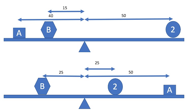Image showing two balanced beams, each with three weights. In the top beam is unknown weight A is a distance of 40 to the left of the fulcrum, unknown weight B is a distance of 15 to the left of the fulcrum and a weight of 2 is 50 to the right of the fulcrum. In the bottom beam is the same unknown weights. Weight A is now a distance of 50 to the right of the fulcrum, weight B is a distance of 25 to the left of the fulcrum and the weight of 2 is a distance of 25 to the right of the fulcrum.

$$40A + 15B = 100$$ $$25B = 50 + 50A$$

As you know, the above system of equations can be written as an Augmented Matrix in the following form:

\[\begin{split} \left[ \begin{matrix} 40 & 15 \\ -50 & 25 \end{matrix} \, \middle\vert \, \begin{matrix} 100 \\ 50 \end{matrix} \right] \end{split}\]

✅ QUESTION: Split apart the augmented matrix ($ \left[ \begin{matrix} A \end{matrix} \, \middle\vert \, \begin{matrix} b \end{matrix} \right] $) into it’s left size ($2 \times 2$) matrix $A$ and it’s right ($2x1$) matrix $b$. Define the matrices $A$ and $b$ as numpy matrices:

#Put your code here

from answercheck import checkanswer

checkanswer.matrix(A,'f5bfd7c52824d5ac580d0ce1ab98fe68');

from answercheck import checkanswer

checkanswer.matrix(b,'c760cd470439f5db82bb165edf4dc3f8');

✅ QUESTION: solve the above system of equations using the np.linalg.solve function and store the value in a vector named x:

# Put your code to the above question here

from answercheck import checkanswer

checkanswer.vector(x,'fc02fe6d0577c4452ee70252e1e17654');

3. Underdetermined Systems¶

Sometimes we have systems of linear equations where we have more unknowns than equations, in this case we call the system “underdetermined.” These types of systems can have infinite solutions. i.e., we can not find an unique $x$ such that $Ax=b$. In this case, we can find a set of equations that represent all of the solutions that solve the problem by using Gauss Jordan and the Reduced Row Echelon form. Lets consider the following example:

\[\begin{split}\begin{bmatrix}5&-2&2 & 1 \\ 4 & -3 &4 &2 \\ 4& -6 &7 & 4\end{bmatrix}\begin{bmatrix}x_1\\x_2\\x_3\\x_4\end{bmatrix}=\begin{bmatrix}1\\2\\3\end{bmatrix}\end{split}\]

✅ QUESTION Define an augmented matrix $M$ that represents the above system of equations:

#Put your code here

✅ QUESTION What is the Reduced Row Echelon form for A?

from answercheck import checkanswer

checkanswer.matrix(M,'efb9b2da0e44984a18f595d7892980e2');

# Put your answer to the above question here

from answercheck import checkanswer

checkanswer.matrix(RREF,'f1fa8baac1df4c378db20cff9e91ca5b');

Notice how the above RREF form of matrix A is different from what we have seen in the past. In this case not all of our values for $x$ are unique. When we write down a solution to this problem by defining the variables by one or more of the undefined variables. for example, here we can see that $x_4$ is undefined. So we say $x_4 = x_4$, i.e. $x_4$ can be any number we want. Then we can define $x_3$ in terms of $x_4$. In this case $x_3 = \frac{11}{15} - \frac{4}{15}x_4$. The entire solution can be written out as follows:

\[\begin{split} \begin{align*} x_1 &= \frac{1}{15} + \frac{1}{15}x_4 \\ x_2 &= \frac{2}{5} + \frac{2}{5}x_4 \\ x_3 &= \frac{11}{15} - \frac{4}{15}x_4 \\ x_4 &= x_4 \end{align*} \end{split}\]

✅ DO THIS Review the above answer and make sure you understand how we get this answer from the Reduced Row Echelon form from above.

Sometimes, in an effort to make the solution more clear, we introduce new variables (typically, $r,s,t$) and substitute them in for our undefined variables so the solution would look like the following:

\[\begin{split} \begin{align*} x_1 &= \frac{1}{15} + \frac{1}{15}r \\ x_2 &= \frac{2}{5} + \frac{2}{5}r \\ x_3 &= \frac{11}{15} - \frac{4}{15}r \\ x_4 &= r \end{align*} \end{split}\]

We can find a particular solution to the above problem by inputing any number for $r$. For example, set r equal to zero and create a vector for all of the $x$ values.

\[\begin{split} \begin{align*} x_1 &= \frac{1}{15}\\ x_2 &= \frac{2}{5}\\ x_3 &= \frac{11}{15} \\ x_4 &= 0 \end{align*} \end{split}\]

##here is the same basic math in python

r = 0
x = np.matrix([1/15+1/15*r, 2/5+2/5*r, 11/15-4/15*r, r]).T
x

✅ DO THIS Define two more matrixes $A$, $b$ representing the above system of equations $Ax=b$:

# put your answer to the above question here.

from answercheck import checkanswer

checkanswer.matrix(A,'a600d0416a3fb9b4bde87b08caf068f1');

from answercheck import checkanswer

checkanswer.vector(b,'4cfaa788e4dd6de04fdf6aea4a0e0e71');

Now let us check our answer by multipying matrix $A$ by our solution $x$ and see if we get $b$

np.allclose(A*x,b)

✅ DO THIS Now go back and pick a different value for $r$ and see that it also produces a valid solution for $Ax=b$.

4. Practice Curve Fitting Example¶

Consider the following polynomial with constant scalars $a$, $b$, and $c$, that falls on the $xy$-plane:

\[f(x) = ax^2 + bx + c\]

✅ QUESTION: Is this function linear? Why or why not?

Put your answer to the above question here.

Assume that we do not know the values of $a$, $b$ and $c$, but we do know that the points (1,2), (-1,12), and (2,3) are on the polynomial. We can substitute the known points into the equation above. For example, using point (1,2) we get the following equation:

\[2 = a1^2 + b1 + c\]

\[\text{or}\]

\[2 = a + b + c\]

✅ QUESTION: Generate two more equations by substituting points (-1,12) and (2,3) into the above equation:

Put your answer to the above question here. (See if you can use latex as I did above)

✅ QUESTION: If we did this right, we should have three equations and three unknowns ($a,b,c$). Note also that these equations are linear (how did that happen?). Transform this system of equations into two matrices $A$ and $b$ like we did above.

#Put your answer to the above question here.

from answercheck import checkanswer

checkanswer.matrix(A,'1896041ded9eebf1cba7e04f32dd1069');

from answercheck import checkanswer

checkanswer.matrix(b,'01e594bb535b4e2f5a04758ff567f918');

✅ QUESTION Write the code to solve for $x$ (i.e., ($a,b,c$)) using numpy.

#Put your answer to the above question here.

from answercheck import checkanswer

checkanswer.vector(x,'1dab22f81c2c156e6adca8ea7ee35dd7');

✅ QUESTION Given the value of your x matrix derived in the previous question, what are the values for $a$, $b$, and $c$?

#Put your answer to the above question here.
a = 0
b = 0
c = 0

Assuming the above is correct, the following code will print your 2nd order polynomial and plot the original points:

x = np.linspace(-3,3)
y = a*x**2 + b*x + c

#plot the function. (Transpose is needed to make the data line up).
plt.plot(x,y.transpose())

#Plot the original points
plt.scatter(1, 2)
plt.scatter(-1, 12)
plt.scatter(2, 3)
plt.xlabel('x-axis')
plt.ylabel('y-axis')

✅ QUESTION The following program is intended to take four points as inputs ($p1, p2, p3, p4 \in R^2$) and calculate the coefficients $a$, $b$, $c$, and $d$ so that the graph of $f(x) = ax^3 + bx^2 + cx + d$ passes smoothly through the points. Test the function with the following points (1,2), (-1,6), (2,3), (3,2) as inputs and print the values for $a$, $b$, $c$, and $d$.

def fitPoly3(p1,p2,p3,p4):
    A = np.matrix([[p1[0]**3, p1[0]**2, p1[0], 1],
                   [p2[0]**3, p2[0]**2, p2[0], 1],
                   [p3[0]**3, p3[0]**2, p3[0], 1],
                   [p4[0]**3, p4[0]**2, p4[0], 1]])
    
    b = np.matrix([p1[1],p2[1],p3[1],p4[1]]).T

    X = np.linalg.solve(A, b)
    a = X[0]
    b = X[1]
    c = X[2]
    d = X[3]
    #Try to put your figure generation code here for the next question 
    #####Start your code here #####
    
    
    #####End of your code here#####       
    return (a,b,c,d)

#put your answer to the above question here

✅ QUESTION Modify the above fitpoly3 function to also generate a figure of the input points and the resulting polynomial in range x=(-3,3).

# Put the answer to the above question above or copy and paste the above function and modify it in this cell. 

✅ QUESTION Give any four $R^2$ input points to fitPoly3, is there always a unique solution? Explain your answer.