08 In-Class Assignment: The Kinematics of Robotics

Image from: https://pixabay.com/images/search/toy robot/
Today, we will calculate the forward kinematics of some 3D robots. This means we would like to come up with a set of transformations such that we can know the \(x,~y,~z\) coordinates of the end effector with respect to the world coordinate system which is at the base of the robot.
1. Review Pre-class Assignment
Like most days, your instructor will review and answer questions from your pre-class assignment. This is your opportunity to ask any lingering questions before the quiz.
2. Pick and Place
Consider the robot depicted in the following image.
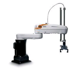
This style of robot is often called a “pick-and-place” robot. It has two motors that rotate around the z-axis to move the end effector in the \(x-y\)-plane; one “linear actuator” which moves up-and-down in the \(z\)-direction; and then finally a third rotating “wrist” joint that turns the “hand” of the robot. Let’s model our robot using the following system diagram:
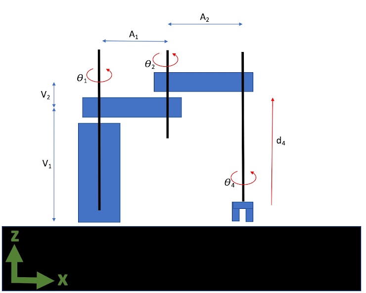
NOTE: The origin for this robot is located at the base of the first “tower” and is in-line with the first joint. The \(x\)-direction goes from the origin to the right and the \(z\)-axis goes from the origin upwards.
This is a little more tricky than the 2D case where everything was rotating around the axes that projects out of the \(x-y\) plane.
In 2D we only really worry about one axis of rotation.
However in 3D we can rotate around the \(x\), \(y\), and \(z\) axis.
The following are the 3D transformation matrices that combine rotation and translations:
X-Axis rotation
Y-Axis rotation
Z-Axis rotation
Question: Construct a joint transformation matrix called \(J_1\), which represents a coordinate system that is located at the top of the first “tower” (robot’s sholder) and moves by rotating around the \(z\)-axis by \(\theta_1\) degrees. Represent your matrix using sympy and the provided symbols:
# Here are some libraries you may need to use
%matplotlib inline
import matplotlib.pylab as plt
import numpy as np
import sympy as sym
import math
sym.init_printing()
---------------------------------------------------------------------------
ModuleNotFoundError                       Traceback (most recent call last)
<ipython-input-1-1e42b50fb0c3> in <module>
      1 # Here are some libraries you may need to use
----> 2 get_ipython().run_line_magic('matplotlib', 'inline')
      3 import matplotlib.pylab as plt
      4 import numpy as np
      5 import sympy as sym

~/REPOS/MTH314_Textbook/MakeTextbook/envs/lib/python3.9/site-packages/IPython/core/interactiveshell.py in run_line_magic(self, magic_name, line, _stack_depth)
   2342                 kwargs['local_ns'] = self.get_local_scope(stack_depth)
   2343             with self.builtin_trap:
-> 2344                 result = fn(*args, **kwargs)
   2345             return result
   2346

~/REPOS/MTH314_Textbook/MakeTextbook/envs/lib/python3.9/site-packages/decorator.py in fun(*args, **kw)
    230             if not kwsyntax:
    231                 args, kw = fix(args, kw, sig)
--> 232             return caller(func, *(extras + args), **kw)
    233     fun.__name__ = func.__name__
    234     fun.__doc__ = func.__doc__

~/REPOS/MTH314_Textbook/MakeTextbook/envs/lib/python3.9/site-packages/IPython/core/magic.py in <lambda>(f, *a, **k)
    185     # but it's overkill for just that one bit of state.
    186     def magic_deco(arg):
--> 187         call = lambda f, *a, **k: f(*a, **k)
    188
    189         if callable(arg):

~/REPOS/MTH314_Textbook/MakeTextbook/envs/lib/python3.9/site-packages/IPython/core/magics/pylab.py in matplotlib(self, line)
     97             print("Available matplotlib backends: %s" % backends_list)
     98         else:
---> 99             gui, backend = self.shell.enable_matplotlib(args.gui.lower() if isinstance(args.gui, str) else args.gui)
    100             self._show_matplotlib_backend(args.gui, backend)
    101

~/REPOS/MTH314_Textbook/MakeTextbook/envs/lib/python3.9/site-packages/IPython/core/interactiveshell.py in enable_matplotlib(self, gui)
   3511         """
   3512         from IPython.core import pylabtools as pt
-> 3513         gui, backend = pt.find_gui_and_backend(gui, self.pylab_gui_select)
   3514
   3515         if gui != 'inline':

~/REPOS/MTH314_Textbook/MakeTextbook/envs/lib/python3.9/site-packages/IPython/core/pylabtools.py in find_gui_and_backend(gui, gui_select)
    278     """
    279
--> 280     import matplotlib
    281
    282     if gui and gui != 'auto':

ModuleNotFoundError: No module named 'matplotlib'
#Use the following symbols

q1,q2,d4,q4,v1,v2,a1,a2 = sym.symbols('\Theta_1, \Theta_2, d_4, \Theta_4, V_1, V_2,A_1,A_2', negative=False)
#put your answer here
q1
Question: Construct a joint transformation matrix called \(J_2\), which represents a coordinate system that is located at the “elbow” joint between the two rotating arms and rotates with the second arm around the \(z\)-axis by \(\theta_2\) degrees. Represent your matrix using sympy and the symbols provided in question a:
#put your answer here
Question: Construct a joint transformation matrix called \(J_3\), which represents a coordinate translation from the “elbow” joint all the way to the horizontal end of the robot arm above the wrist joint. Note: there is no rotation in this transformation. Represent your matrix using sympy and the symbols provided in question a:
#put your answer here
Question: Construct a joint transformation matrix called \(J_4\), which represents a coordinate system that is located at the tip of the robot’s “hand” and rotates around the \(z\)-axis by \(\theta_4\). This one is a little different, the configuration is such that the hand touches the table when \(d_4=0\) so the translation component for the matrix in the z axis is \(d_4-V_1-V_2\).
#put your answer here
Question: Rewrite the joint transformation matrices from questions a - d as numpy matrices with discrete (instead of symbolic) values. Plug in your transformations in the code below and use this to simulate the robot:
from ipywidgets import interact
from mpl_toolkits.mplot3d import Axes3D

def Robot_Simulator(theta1=0,theta2=-0,d4=0,theta4=0):

    #Convert from degrees to radians
    q1 = theta1/180 * math.pi
    q2 = theta2/180 * math.pi
    q4 = theta4/180 * math.pi

    #Define robot geomitry
    V1 = 4
    V2 = 0
    A1 = 2
    A2 = 2

    #Define your transfomraiton matrices here.
    J1 = np.matrix([[1, 0, 0, 0 ],
                    [0, 1, 0, 0 ],
                    [0, 0, 1, 0],
                    [0, 0, 0, 1]])

    J2 = np.matrix([[1, 0, 0, 0 ],
                    [0, 1, 0, 0 ],
                    [0, 0, 1, 0],
                    [0, 0, 0, 1]])

    J3 = np.matrix([[1, 0, 0, 0 ],
                    [0, 1, 0, 0 ],
                    [0, 0, 1, 0],
                    [0, 0, 0, 1]])

    J4 = np.matrix([[1, 0, 0, 0 ],
                    [0, 1, 0, 0 ],
                    [0, 0, 1, 0],
                    [0, 0, 0, 1]])


    #Make the rigid end effector
    p = np.matrix([[-0.5,0,0, 1], [-0.5,0,0.5,1], [0.5,0,0.5, 1], [0.5,0,0,1],[0.5,0,0.5, 1], [0,0,0.5,1], [0,0,V1+V2,1]]).T

    #Propogate and add joint points though the simulation
    p = np.concatenate((J4*p, np.matrix([0,0,0,1]).T), axis=1 )
    p = np.concatenate((J3*p, np.matrix([0,0,0,1]).T), axis=1 )
    p = np.concatenate((J2*p, np.matrix([0,0,0,1]).T), axis=1 )
    p = np.concatenate((J1*p, np.matrix([0,0,0,1]).T), axis=1 )

    fig = plt.figure()
    ax = fig.add_subplot(111, projection='3d')

    ax.scatter(p[0,:].tolist()[0],(p[1,:]).tolist()[0], (p[2,:]).tolist()[0], s=20, facecolors='blue', edgecolors='r')
    ax.scatter(0,0,0, s=20, facecolors='r', edgecolors='r')
    ax.plot(p[0,:].tolist()[0],(p[1,:]).tolist()[0], (p[2,:]).tolist()[0])
    ax.set_xlim([-5,5])
    ax.set_ylim([-5,5])
    ax.set_zlim([0,6])
    ax.set_xlabel('x-axis')
    ax.set_ylabel('y-axis')
    ax.set_zlabel('z-axis')

    plt.show()

target = interact(Robot_Simulator, theta1=(-180,180), theta2=(-180,180), d4=(0,6), theta4=(-180,180)); ##TODO: Modify this line of code
✅ Question: Can we change the order of the transformation matrices? Why? You can try and see what happens.
Put your answer to the above question here.
3. Odd Clock
Consider the clock depicted in the following image.

from: Hackaday
Instead of a standard clock–which has independent hour and minute hands–this clock connects the minute hand at the end of the hour hand. Here is a video showing the sped-up clock motion:
from IPython.display import YouTubeVideo
YouTubeVideo("bowLiSlm_gA",width=640,height=360, mute=1)
The following code is an animated traditional clock which uses the function as a trick to animate things in jupyter:
%matplotlib inline
import matplotlib.pylab as plt
from IPython.display import display, clear_output
import time
def show_animation(delay=0.01):
    fig = plt.gcf();
    time.sleep(delay)       # Sleep for half a second to slow down the animation
    clear_output(wait=True) # Clear output for dynamic display
    display(fig)            # Reset display
    fig.clear()             # Prevent overlapping and layered plots
Lets see a standard analog clock run at high speed
import numpy as np
'''
Analog clock plotter with time input as seconds
'''
def analog_clock(tm=0):

    #Convert from time to radians
    a_minutes = -tm/(60*60) * np.pi * 2
    a_hours = -tm/(60*60*12) * np.pi * 2

    #Define clock hand sizees
    d_minutes = 4
    d_hours = 3
    arrow_width=0.5
    arrow_length=1

    # Set up figure
    fig = plt.gcf()
    ax = fig.gca();
    ax.set_xlim([-15,15]);
    ax.set_ylim([-10,10]);
    ax.scatter(0,0, s=15000, color="navy"); #Background Circle
    plt.axis('off');

    # Calculation Minute hand transformation matrix
    J2 = np.matrix([[np.cos(a_minutes), -np.sin(a_minutes)],
                    [np.sin(a_minutes), np.cos(a_minutes)]] )
    pm = np.matrix([[0,d_minutes], [-arrow_width,d_minutes], [0,arrow_length+d_minutes], [arrow_width,d_minutes], [0,d_minutes]] ).T;
    pm = np.concatenate((J2*pm, np.matrix([0,0]).T), axis=1 );
    ax.plot(pm[0,:].tolist()[0],(pm[1,:]).tolist()[0], color='cyan', linewidth=2);

    # Calculation Hour hand transformation matrix
    J1 = np.matrix([[np.cos(a_hours), -np.sin(a_hours)],
                    [np.sin(a_hours), np.cos(a_hours)]] )
    ph = np.matrix([[0,d_hours], [0,d_hours], [-arrow_width,d_hours], [0,arrow_length+d_hours], [arrow_width,d_hours], [0,d_hours]]).T;
    ph = np.concatenate((J1*ph, np.matrix([0,0]).T), axis=1 );
    ax.plot(ph[0,:].tolist()[0],(ph[1,:]).tolist()[0], color='yellow', linewidth=2);
#Run the clock for about 5 hours at 100 times speed so we can see the hands move
for tm in range(0,60*60*5, 100):
    analog_clock(tm);
    show_animation();
For the following few questions, consider the transformation matrix \(J_1\) redefined below with an angle of 5 hours out of 12.
import sympy as sym
import numpy as np
sym.init_printing(use_unicode=True)

a_hours = 5/12 * 2 * np.pi
J1 = np.matrix([[np.cos(a_hours), -np.sin(a_hours)],
                [np.sin(a_hours), np.cos(a_hours)]] )

sym.Matrix(J1)
✅ Question: Using code, show that the transpose of \(J_1\) is also the inverse of \(J_1\), then explain how the code demonstrates the answer.
#Put your answer here
Explain your answer here.
✅ Question: Given the trigonometric identity \(cos^2(\theta) + sin^2(\theta) = 1\), prove by construction–using either Python or \(\LaTeX\)/Markdown or sympy (if you are feeling adventurous)–that the transpose of the \(J_1\) matrix is also the inverse for ANY angle a_hours \(\in [0, 2\pi]\).
Put your prof here.
Now consider the following code which attempts to connect the hands on the clock together to make the Odd Clock shown in the video above.
%matplotlib inline
import matplotlib.pylab as plt
from IPython.display import display, clear_output
import time
def show_animation(delay=0.01):
    fig = plt.gcf();
    time.sleep(delay)       # Sleep for half a second to slow down the animation
    clear_output(wait=True) # Clear output for dynamic display
    display(fig)            # Reset display
    fig.clear()             # Prevent overlapping and layered plots
import numpy as np

def odd_clock(tm=0):

    #Convert from time to radians
    #a_seconds = -tm/60 * np.pi * 2
    a_minutes = -tm/(60*60) * np.pi * 2
    a_hours = -tm/(60*60*12) * np.pi * 2

    #Define robot geomitry
    #d_seconds = 2.5
    d_minutes = 2
    d_hours = 1.5
    arrow_width=0.5
    arrow_length=1

    # Set up figure
    fig = plt.gcf()
    ax = fig.gca();
    ax.set_xlim([-15,15]);
    ax.set_ylim([-10,10]);
    plt.axis('off');

    #Define the arrow at the end of the last hand
    #p = np.matrix([[0,d_minutes,1], [0,0,1]]).T
    p = np.matrix([[0,d_minutes,1], [-arrow_width,d_minutes,1], [0,arrow_length+d_minutes,1], [arrow_width,d_minutes,1 ], [0,d_minutes,1 ], [0,0,1]] ).T;

    # Calculation Second hand transformation matrix
    J2 = np.matrix([[np.cos(a_minutes), -np.sin(a_minutes), 0 ],
                    [np.sin(a_minutes), np.cos(a_minutes), d_hours ],
                    [0, 0, 1]])
    p = np.concatenate((J2*p, np.matrix([0,0,1]).T), axis=1 )

    J1 = np.matrix([[np.cos(a_hours), -np.sin(a_hours), 0 ],
                    [np.sin(a_hours), np.cos(a_hours), 0 ],
                    [0, 0, 1]])
    p = np.concatenate((J1*p, np.matrix([0,0,1]).T), axis=1 )

    ax.scatter(0,0, s=20, facecolors='r', edgecolors='r')
    ax.plot(p[0,:].tolist()[0],(p[1,:]).tolist()[0])
#Run the clock for about 5 hours at 100 times speed so we can see the hands move
for tm in range(0,60*60*5, 100):
    odd_clock(tm);
    show_animation();
✅ Question: Using the given point (\(p\)) written in “minutes” coordinates (on line 26 of the above code) and the above transformation matrices (\(J_1,J_2\)), write down the equation to transform \(p\) into world coordinates \(p_w\).
Put the answer to the above question here
✅ Question: Notice the above odd_clock function has variables d_seconds and a_seconds commented out. Use these variables and modify the above code to add a “seconds” hand on the tip of the minute hand such that the seconds hand moves around the minute hand just like the minute hand moves around the hour hand. If you have trouble, use the following cell to explain your thought process and where you are getting stuck.
Written by Dr. Dirk Colbry, Michigan State University

This work is licensed under a Creative Commons Attribution-NonCommercial 4.0 International License.