06 In-Class Assignment: Matrix Multiply
![Image showing how matrix multiply works. There is a 2 by 3 matrix multiplied by a 3 by 2 matrix to get a 2 by 2 matrix. The first row in the first matrix is highlighted and the first column of the second matrix is highlighted. The words 'Dot Product' are pointing to the highlighted row and column and the single value output is shown in as the only element in the upper left of the 2 by 2 result. Basically the image is showing that the row [1,2,3] dotted with the column [7,9,11] results in the single output of 58.](https://www.mathsisfun.com/algebra/images/matrix-multiply-a.svg)
Image from: www.mathsisfun.com
Agenda for today’s class (80 minutes)
(20 minutes) Review of Pre class assignment
(30 minutes) Systems of Linear Equations with Many Solutions
(30 minutes) Matrix Multiply
2. Systems of Linear Equations with Many Solutions
When we solve a system of equations of the form \(Ax=b\), we mentioned that we may have three outcomes:
a unique solution
no solution
infinity many solutions
Assume that we have \(m\) equations and \(n\) unkowns.
Case 1 \(m < n\), we do not have enough equations, there will be only TWO outcomes: no solution, or infinity many solutions.
Case 2 \(m = n\), we may have all THREE outcomes. If the determinant is nonzero, we have a unique solution, otherwise, we have to decide the outcome based on the augmented matrix.
Case 3 \(m>n\), we have more equations than the number of unknowns. That means there will be redundant equations (we can remove them) or conflict equations (no solution). We may have all THREE outcomes.
We talked about several methods for solving the system of equations. The most general one is the Gauss-Jordan or Gaussian elimination, which works for all three cases. Note that Jacobian and Gauss-Seidel can not work on Case 1 and Case 3.
We will focus on the Gaussian elimination. After the Gaussian elimiation, we look at the last several rows (could be zero) with all zeros except the last column.
If one element from the corresponding right hand side is not zero, we have that \(0\) equals some nonzero number, which is impossible. Therefore, there is no solution. E.g.,
In this case, we say that the system is inconsistent. Later in the semester we will look into methods that try to find a “good enough” solution for an inconsistant system (regression).
Otherwise, we remove all the rows with all zeros (which is the same as removing redundant equations). If the number of remaining equations is the same as the number of unknowns, the rref is an identity matrix, and we have unique solution. E.g., $\(\left[ \begin{matrix} 1 & 0 & 0 \\ 0 & 1 & 0 \\ 0 & 0 & 1 \\ 0 & 0 & 0 \end{matrix} \, \middle\vert \, \begin{matrix} 2 \\ 3 \\ 4 \\ 0 \end{matrix} \right] \Rightarrow \left[ \begin{matrix} 1 & 0 & 0 \\ 0 & 1 & 0 \\ 0 & 0 & 1 \\ \end{matrix} \, \middle\vert \, \begin{matrix} 2 \\ 3 \\ 4 \end{matrix} \right] \)$
If the number of remaining equations is less than the number of unknowns, we have infinitely many solutions. Consider the following three examples:
where \(x_3\) is a free variable.
where \(x_2\) is a free variable.
where \(x_2\) and \(x_4\) are free variables.
✅ QUESTION: Assume that the system is consistent, explain why the number of equations can not be larger than the number of unknowns after the redundant equations are removed?
Put the solution to the above question here.
✅ DO THIS: If there are two solutions for \(Ax=b\), that is \(Ax=b\) and \(Ax'=b\) while \(x\neq x'\). Check that \(A(cx+(1-c)x') = b\) for any real number \(c\). Therefore, if we have two different solutions, we have infinite many solutions.
Put the solution to the above question here.
If \(Ax=b\) and \(Ax'=b\), then we have \(A(x-x')=0\). If \(x\) is a particular solution to \(Ax=b\), then all the solutions to \(Ax=b\) are \(\{x+v: v \mbox{ is a solution to the homogeneous system } Av=0\}\).
The solution for \(Ax=0\) is always a subspace.
After removing the redundant rows, if the number of equations is the same as the number of unknowns, we have a unique solution. If the difference between the number of equations and the number of unknowns is 1, all the solutions lie on a line. If the difference is 2, all the solutions lie on a 2-D plane.
✅ QUESTION: What is the solution to the following set of linear equations in augmented matrix form?
Put the solution to the above question here.
3. Matrix Multiply
✅ DO THIS: Write your own matrix multiplication function using the template below and compare it to the built-in matrix multiplication that can be found in numpy. Your function should take two “lists of lists” as inputs and return the result as a third list of lists.
#some libraries (maybe not all) you will need in this notebook
%matplotlib inline
import matplotlib.pylab as plt
import numpy as np
import sympy as sym
sym.init_printing(use_unicode=True)

import random
import time
---------------------------------------------------------------------------
ModuleNotFoundError                       Traceback (most recent call last)
<ipython-input-1-f8d5de0eda7c> in <module>
      1 #some libraries (maybe not all) you will need in this notebook
----> 2 get_ipython().run_line_magic('matplotlib', 'inline')
      3 import matplotlib.pylab as plt
      4 import numpy as np
      5 import sympy as sym

~/REPOS/MTH314_Textbook/MakeTextbook/envs/lib/python3.9/site-packages/IPython/core/interactiveshell.py in run_line_magic(self, magic_name, line, _stack_depth)
   2342                 kwargs['local_ns'] = self.get_local_scope(stack_depth)
   2343             with self.builtin_trap:
-> 2344                 result = fn(*args, **kwargs)
   2345             return result
   2346

~/REPOS/MTH314_Textbook/MakeTextbook/envs/lib/python3.9/site-packages/decorator.py in fun(*args, **kw)
    230             if not kwsyntax:
    231                 args, kw = fix(args, kw, sig)
--> 232             return caller(func, *(extras + args), **kw)
    233     fun.__name__ = func.__name__
    234     fun.__doc__ = func.__doc__

~/REPOS/MTH314_Textbook/MakeTextbook/envs/lib/python3.9/site-packages/IPython/core/magic.py in <lambda>(f, *a, **k)
    185     # but it's overkill for just that one bit of state.
    186     def magic_deco(arg):
--> 187         call = lambda f, *a, **k: f(*a, **k)
    188
    189         if callable(arg):

~/REPOS/MTH314_Textbook/MakeTextbook/envs/lib/python3.9/site-packages/IPython/core/magics/pylab.py in matplotlib(self, line)
     97             print("Available matplotlib backends: %s" % backends_list)
     98         else:
---> 99             gui, backend = self.shell.enable_matplotlib(args.gui.lower() if isinstance(args.gui, str) else args.gui)
    100             self._show_matplotlib_backend(args.gui, backend)
    101

~/REPOS/MTH314_Textbook/MakeTextbook/envs/lib/python3.9/site-packages/IPython/core/interactiveshell.py in enable_matplotlib(self, gui)
   3511         """
   3512         from IPython.core import pylabtools as pt
-> 3513         gui, backend = pt.find_gui_and_backend(gui, self.pylab_gui_select)
   3514
   3515         if gui != 'inline':

~/REPOS/MTH314_Textbook/MakeTextbook/envs/lib/python3.9/site-packages/IPython/core/pylabtools.py in find_gui_and_backend(gui, gui_select)
    278     """
    279
--> 280     import matplotlib
    281
    282     if gui and gui != 'auto':

ModuleNotFoundError: No module named 'matplotlib'
def multiply(m1,m2):
    #first matrix is nxd in size
    #second matrix is dxm in size
    n = len(m1)
    d = len(m2)
    m = len(m2[0])

    #check to make sure sizes match
    if len(m1[0]) != d:
        print("ERROR - inner dimentions not equal")

    #### put your matrix multiply code here #####

    return result
Test your code with the following examples
#Basic test 1
n = 3
d = 2
m = 4

#generate two random lists of lists.
matrix1 = [[random.random() for i in range(d)] for j in range(n)]
matrix2 = [[random.random() for i in range(m)] for j in range(d)]
sym.init_printing(use_unicode=True) # Trick to make matrixes look nice in jupyter

sym.Matrix(matrix1) # Show matrix using sympy
sym.Matrix(matrix2) # Show matrix using sympy
#Compute matrix multiply using your function
x = multiply(matrix1, matrix2)
#Compare to numpy result
np_x = np.matrix(matrix1)*np.matrix(matrix2)

#use allclose function to see if they are numrically "close enough"
print(np.allclose(x, np_x))

#Result should be True
#Test identity matrix
n = 4

# Make a Random Matrix
matrix1 = [[random.random() for i in range(n)] for j in range(n)]
sym.Matrix(matrix1) # Show matrix using sympy
#generate a 3x3 identity matrix
matrix2 = [[0 for i in range(n)] for j in range(n)]
for i in range(n):
    matrix2[i][i] = 1
sym.Matrix(matrix2) # Show matrix using sympy
result = multiply(matrix1, matrix2)

#Verify results are the same as the original
np.allclose(matrix1, result)
Timing Study
In this part, you will compare your matrix multiplication with the numpy matrix multiplication.
You will multiply two randomly generated \(n\times n\) matrices using both the multiply() function defined above and the numpy matrix multiplication.
Here is the basic structure of your timing study:
Initialize two empty lists called
my_timeandnumpy_timeLoop over values of n (100, 200, 300, 400, 500)
For each value of \(n\) use the time.clock() function to calculate the time it takes to use your algorithm and append that time (in seconds) to the
my_timelist.For each value of \(n\) use the time.clock() function to calculate the time it takes to use the
numpymatrix multiplication and append that time (in seconds) to thenumpy_timelist.Use the provided code to generate a scatter plot of your results.
n_list = [100, 200, 300, 400, 500]
my_time = []
numpy_time = []
# RUN AT YOUR OWN RISK.
# THIS MAY TAKE A WHILE!!!!

for n in n_list:
    print(f"Measureing time it takes to multiply matrixes of size {n}")
    #Generate random nxn array of two lists
    matrix1 = [[random.random() for i in range(n)] for j in range(n)]
    matrix2 = [[random.random() for i in range(n)] for j in range(n)]
    start = time.time()
    x = multiply(matrix1, matrix2)
    stop = time.time()
    my_time.append(stop - start)

    #Convert the lists to a numpy matrix
    npm1 = np.matrix(matrix1)
    npm2 = np.matrix(matrix2)

    #Calculate the time it takes to run the numpy matrix.
    start = time.time()
    answer = npm1*npm2
    stop = time.time()
    numpy_time.append(stop - start)
plt.scatter(n_list,my_time, color='red', label = 'my time')
plt.scatter(n_list,numpy_time, color='green', label='numpy time')

plt.xlabel('Size of $n x n$ matrix');
plt.ylabel('time (seconds)')
plt.legend();
Based on the above results, you can see that the numpy algorithm not only is faster but also “scales” at a slower rate than your algorithm.
✅ QUESTION: Why do you think the numpy matrix multiplication is so much faster?
Put your answer to the above question here